For a while now I have been advocating for tuning ε in various parts of the modern deep learning stack, and in this post I’ll explain why.
What do I mean by ε?
The fifth letter in the Greek alphabet, ε is usually a nuisance parameter in many modern deep learning techniques. Often inserted in a denominator to avoid division by zero, it is a very small positive constant that is almost always left unchanged, or if it is changed then this fact is not widely appreciated.
This post was motivated by a recent Twitter thread where many people were (understandably) surprised at the large change in performance when changing ε from 10-7 to 10-5 in RMSProp in an A2C RL experiment, but this wasn't the first social media post to wonder about this often forgotten parameter.
Adam, RMSProp, Ada*
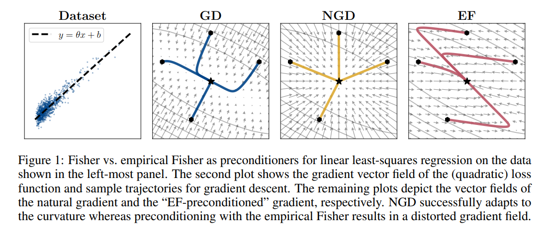
In many preconditioned optimizers (Adam, RMSProp, AdaGrad, K-FAC, Shampoo, etc.), there is a multiple of the identity matrix added to the preconditioning matrix before inverting it. In Adam and RMSProp (and the too many variations of them that have recently come up, see Appendix A of [12]), this preconditioning matrix is (approximately) the diagonal of the empirical Fisher matrix (see [15] for a great analysis of the empirical vs true Fishers), and so this ε hyperparameter is just added elementwise to the second moment estimates. Often times this is done to avoid numerical issues with inverting (dividing by) the preconditioner. This works because we know the minimum eigenvalue of the matrix (P + εI) is the mininum eigenvalue of P plus ε, so as long as ε is larger than any negative eigenvales of P then we will have a positive definite matrix which we can invert (the same logic applies with diagonal preconditioners, just with division by zero instead of matrix inversion). See [19] for a discussion of the numerical challenges involved in preconditioned optimization. In addition to this very useful feature, we can also decompose ε into serving another purpose as part of a trust region radius on the optimizer updates (the actual trust region radius depends on both ε and our preconditioner).

A comparison of preconditioners, from [15].
In each the optimizers listed above, the preconditioner being applied is only an approximation to the true curvature of the loss surface we are optimizing (and are usually derived via second-order Taylor expansions around the current loss). As expected, the approximation will become less accurate the further away we move from the current value of the parameters, and if the approximation is very bad then we may not have to move very far for it to break down. Ideally, the preconditioning would be weaker when we are less confident in its accuracy; luckily, ε gives us a way to control this! Simply put, the larger ε is, the smaller the effect of the preconditioner on our optimizer's update. However, we want to also keep ε, sometimes referred to as damping in this context, as small as possible, because as mentioned above it will get rid of low curvature (small eigenvalue) directions in the preconditioning that are useful to consider when speeding up optimization.
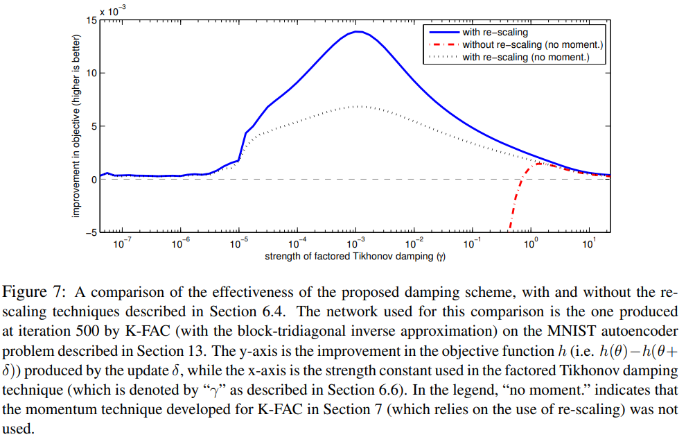
One way to strike a balance between keeping ε small enough to keep low curavture directions around, but also large when we are not confident in our preconditioner approximation, is to change ε during optimization. One way to achieve this is via a heuristic used in the Levenberg-Marquardt algorithm. Put simply, we calculate how much our loss function changed between two updates, and compare this to how much a second-order Taylor expansion of the loss predicted it should change, and if the two are in agreement then we can have confidence in our preconditioner (note that we can use Hessian-vector products to compute the second order term in our Taylor expansion). Each time we calculate this, we increase or decrease the damping (ε) term by a multiplicative factor; see section 6 of the KFAC paper [13] for a more detailed explanation. In the beginning of training, our approximations to the loss surface curvature will likely be very bad: we have not yet warmed up our gradient exponential moving averages used in calculating it, and the loss surface characteristic are changing more rapidly then they will be when we are closer to the optimum, which we usually assume is a well behaved quadratic. Conversely, we want to have the preconditioner have access to as many low curvature directions as possible towards the end of optimization, so we can more accurately pinpoint the bottom of the optimum. While it is not guaranteed that ε will monotonically decrease throughout training with the scheme described above, in my experience on common benchmark problems (ResNets on CIFAR/ImageNet) this rule almost always decreases ε. Therefore I would actually recommend using an exponential decay schedule for ε instead of a fixed value, where the final value is extremely close to zero.

An analysis of the effect of damping strength in KFAC on an MNIST autoencoder, from [13].
One reason why the effects of ε may not have been noticed much in popular optimizers such as Adam and RMSProp is because they use a square root around their second moment estimates of the gradients, which can be viewed as a non-linear version of damping; once the numerics of dividing by zero have been solved by ε, the square root can handle diminishinig large dimensions and increasing small ones, which will have a similar normalizing effect on the eigenvalues. In fact, if you are feeling adventurous, tuning the exponent in Adam and RMSProp to be something other than 1/2 could possibly yield additional improvements.
Finally, for some experiments there exists an interesting relationship betweeen ε and weight decay, as thoroughly outlined in [14]. Put simply, under various conditions discussed in [14], the scale of the weights affects the scale of the gradients which affects our preconditioning matrix. Thus, the scale of the weights will affect the balance between our preconditioner matrix and our damping term ε, and so weight decay can interact with ε through this process. Therefore, it may be useful to jointly tune of ε and weight decay, beyond the effect that they both have on the effective learning rate of an update.
Batch Norm

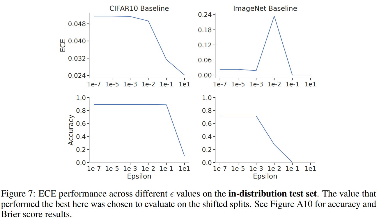
Demonstrating the effect of ε in Batch Norm on model calibration, from [17].
Batch Normalization is an ever-present and ever-annoying improvement to many deep learning pipelines. It too has an ε parameter, which is used in the denominator of its normalization to avoid dividing by a zero-valued variance. One key thing to note is that Batch Norm is oftentimes applied channelwise to convolutional layers, and so by increasing the ε in the denominator we are effectively temperature scaling/smoothing out the differences in magnitude across activation channels. In addition to these potential normalization benefits which are similar to Local Response Normalization[16], this could also have an effect on the entropy of the model's output distribution. In many architectures, the Batch Norm normalized channel activations are averaged into a final vector that is put through a linear layer to obtain the model logits; therefore, if the activations going into the final average pooling layer are closer together in value, the final linear layer will have to explicitly learn to make them separate in value again. While this could happen, we did see in [17] that increasing ε in Batch Norm improved model calibration, as measured by Expected Calibration Error, especially on CIFAR10 (before destroying model accuracy.)
Implementation differences
It is also interesting to look at how different implementations of (supposedly) the same algorithms choose different default values for ε.
The TensorFlow documentation for Adam is the only one to mention that using default ε values may not always be the best choice: "The default value of 1e-7 for epsilon might not be a good default in general. For example, when training an Inception network on ImageNet a current good choice is 1.0 or 0.1.". However, we should note that the default value is 10-7 for tf.keras.optimizers.Adam and 10-8 for tf.train.AdamOptimizer, PyTorch and Flax.
Regarding Batch Normalization, the TensorFlow layer uses a default ε = 10-3 whereas Flax and PyTorch both use default ε = 10-5. Note that often times, ImageNet/ResNet-50 pipelines will explicitly specify a Batch Norm ε = 10-5.
Another potential framework difference is whether or not epsilon is added before or after taking the square root of the diagonal Fisher. This has been previously pointed out for RMSProp in TF vs PyTorch, where PyTorch adds ε after the square root and TF adds it inside the square root, but it should also be noted that if momentum is not used in RMSProp in TF then ε is added outside the square root again! Hinton's course slides that introduced RMSProp did not specify anything about ε.
There also exist differences in ε defaults for AdaGrad, as originally pointed out in Appendix B of [11]; tf.keras.optimizers.Adagrad defaults to ε = 10-7, while tf.train.AdagradOptimizer defaults to ε = 0.1. In PyTorch the default ε is 10-10, and Flax uses a default ε = 10-8.
Previous works
It is actually more common to use non-default values than many realize (many references taken from our paper[1]), as seen in the following previous works:
- [2] considers ε = 10-3 and note that it can be viewed as an adaptivity parameter to diminish the effect of the velocity in Adam.
- [3] (which introduces RAdam) considers ε = 10-4 to reduce the variance of the adaptive learning rate of Adam.
- [4] uses ε = 10-6 in Adam for pretraining their RoBERTa models.
- [5] includes an analysis of Adam and RMSProp hyperparameters and finds that they can both be sensitive to ε.
- [6] (which introduces Inception-v2) uses an ε = 1.0 for RMSProp to train their models.
- [7] (which introduces the Rainbow RL technique) uses an ε = 1.5 x 10⁻⁴ for Adam to train their models.
- [8, 9] (MnasNet, EfficientNet) use ε = 10-3 in RMSProp but do not mention so in the papers, but can be found in their code.
- the original DQN code from DeepMind uses ε = 0.01 in RMSProp.
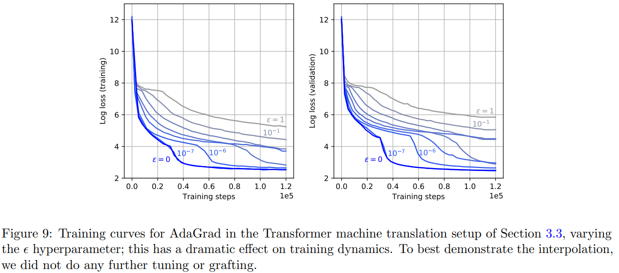
- [10] (learning rate grafting) sweeps over ε values in [0, 1] for AdaGrad and finds that it can have a noticeable impact on training performance.

An analysis of the effect of ε in AdaGrad on a Transformer, from [10].
Parting advice
As models are getting larger and larger, hyperparameter tuning is getting more and more expensive. While I agree with a lot of the existing literature[18] on tuning the learning rate and learning rate schedule first, I also believe that if you can afford it, when tuning optimizers trying one or two values of ε that is a few orders of magnitude larger than the default can be useful. For example, I would try both the default values and ε = 10-3 for Adam or RMSProp in your searches. If possible, an exponential decay from the initial value to some value very very close to zero could provide even more benefits!
If you can afford even more trials, I would also recommend tuning ε on a floating point or grid search log scale. Even better, jointly tuning the learning rate and/or weight decay with ε, as we did in [1], can help take into account the ways which the hyperparameters affect one another.
While not as impactful, one can still improve model performance by tuning the Batch Norm ε, namely increasing it can lead to slightly improved model calibration (although I would recommend many other calibration improvement techniques first).
In the end, I believe all of this evidence goes to show that optimizer hyperparameter tuning can have dramatic effects on model performance, and so it should always be done with care and deliberation (and more importantly, always detailed in any resulting papers!)
References
- [1] On Empirical Comparisons of Optimizers for Deep Learning
- Dami Choi, Christopher J. Shallue, Zachary Nado, Jaehoon Lee, Chris J. Maddison, George E. Dahl
- https://arxiv.org/abs/1910.05446
- [2] Adaptive Methods for Nonconvex Optimization
- Manzil Zaheer, Sashank Reddi, Devendra Sachan, Satyen Kale, Sanjiv Kumar
- https://papers.nips.cc/paper/2018/hash/90365351ccc7437a1309dc64e4db32a3-Abstract.html
- [3] On the Variance of the Adaptive Learning Rate and Beyond
- Liyuan Liu, Haoming Jiang, Pengcheng He, Weizhu Chen, Xiaodong Liu, Jianfeng Gao, Jiawei Han
- https://arxiv.org/abs/1908.03265
- [4] RoBERTa: A Robustly Optimized BERT Pretraining Approach
- Yinhan Liu, Myle Ott, Naman Goyal, Jingfei Du, Mandar Joshi, Danqi Chen, Omer Levy, Mike Lewis, Luke Zettlemoyer, Veselin Stoyanov
- https://arxiv.org/abs/1907.11692
- [5] Convergence guarantees for RMSProp and ADAM in non-convex optimization and an empirical comparison to Nesterov acceleration
- Soham De, Anirbit Mukherjee, Enayat Ullah
- https://arxiv.org/abs/1807.06766
- [6] Rethinking the Inception Architecture for Computer Vision
- Christian Szegedy, Vincent Vanhoucke, Sergey Ioffe, Jonathon Shlens, Zbigniew Wojna
- https://arxiv.org/abs/1512.00567
- [7] Rainbow: Combining Improvements in Deep Reinforcement Learning
- Matteo Hessel, Joseph Modayil, Hado van Hasselt, Tom Schaul, Georg Ostrovski, Will Dabney, Dan Horgan, Bilal Piot, Mohammad Azar, David Silver
- https://arxiv.org/abs/1710.02298
- [8] MnasNet: Platform-Aware Neural Architecture Search for Mobile
- Mingxing Tan, Bo Chen, Ruoming Pang, Vijay Vasudevan, Mark Sandler, Andrew Howard, Quoc V. Le
- https://arxiv.org/abs/1807.11626
- [9] EfficientNet: Rethinking Model Scaling for Convolutional Neural Networks
- Mingxing Tan, Quoc V. Le
- https://arxiv.org/abs/1905.11946
- [10] Disentangling Adaptive Gradient Methods from Learning Rates
- Naman Agarwal, Rohan Anil, Elad Hazan, Tomer Koren, Cyril Zhang
- https://arxiv.org/abs/2002.11803
- [11] The Marginal Value of Adaptive Gradient Methods in Machine Learning
- Ashia C. Wilson, Rebecca Roelofs, Mitchell Stern, Nathan Srebro, Benjamin Recht
- https://arxiv.org/abs/1705.08292
- [12] Descending through a Crowded Valley -- Benchmarking Deep Learning Optimizers
- Robin M. Schmidt, Frank Schneider, Philipp Hennig
- https://arxiv.org/abs/2007.01547
- [13] Optimizing Neural Networks with Kronecker-factored Approximate Curvature
- James Martens, Roger Grosse
- https://arxiv.org/abs/1503.05671
- [14] Three Mechanisms of Weight Decay Regularization
- Guodong Zhang, Chaoqi Wang, Bowen Xu, Roger Grosse
- https://arxiv.org/abs/1810.12281
- [15] Limitations of the Empirical Fisher Approximation for Natural Gradient Descent
- Frederik Kunstner, Lukas Balles, Philipp Hennig
- https://arxiv.org/abs/1905.12558
- [16] ImageNet Classification with Deep Convolutional Neural Networks
- Alex Krizhevsky, Ilya Sutskever, Geoffrey E. Hinton
- https://papers.nips.cc/paper/2012/file/c399862d3b9d6b76c8436e924a68c45b-Paper.pdf
- [17] Evaluating Prediction-Time Batch Normalization for Robustness under Covariate Shift
- Zachary Nado, Shreyas Padhy, D. Sculley, Alexander D'Amour, Balaji Lakshminarayanan, Jasper Snoek
- https://arxiv.org/abs/2006.10963
- [18] Optimizer Benchmarking Needs to Account for Hyperparameter Tuning
- Prabhu Teja S, Florian Mai, Thijs Vogels, Martin Jaggi, François Fleuret
- https://arxiv.org/abs/1910.11758
- [19] Second Order Optimization Made Practical
- Rohan Anil, Vineet Gupta, Tomer Koren, Kevin Regan, Yoram Singer
- https://arxiv.org/abs/2002.09018